How to Derive Logistic Growth

Separation of Variables

Separate variables. 1 P ( 1 − P L ) d P = k d t {\displaystyle {\frac {1}{P\left(1-{\frac {P}{L}}\right)}}\mathrm {d} P=k\mathrm {d} t} {\frac {1}{P\left(1-{\frac {P}{L}}\right)}}{\mathrm {d}}P=k{\mathrm {d}}t

Decompose into partial fractions. Since the denominator on the left side has two terms, we need to separate them for easy integration. Multiply the left side by L L {\displaystyle {\frac {L}{L}}} {\frac {L}{L}} and decompose. L L P − P 2 d P = L P ( L − P ) d P = A P d P + B L − P d P {\displaystyle {\begin{aligned}{\frac {L}{LP-P^{2}}}\mathrm {d} P&={\frac {L}{P(L-P)}}\mathrm {d} P\\&={\frac {A}{P}}\mathrm {d} P+{\frac {B}{L-P}}\mathrm {d} P\end{aligned}}} {\begin{aligned}{\frac {L}{LP-P^{{2}}}}{\mathrm {d}}P&={\frac {L}{P(L-P)}}{\mathrm {d}}P\\&={\frac {A}{P}}{\mathrm {d}}P+{\frac {B}{L-P}}{\mathrm {d}}P\end{aligned}} Solve for A {\displaystyle A} A and B . {\displaystyle B.} B. L = A ( L − P ) + B P , let L = 0 {\displaystyle L=A(L-P)+BP,\ {\text{let }}L=0} L=A(L-P)+BP,\ {\text{let }}L=0 0 = − A P + B P , A = B {\displaystyle 0=-AP+BP,\ A=B} 0=-AP+BP,\ A=B let P = 0 : L = A L {\displaystyle {\text{let }}P=0:L=AL} {\text{let }}P=0:L=AL A = 1 , B = 1 {\displaystyle A=1,\ B=1} A=1,\ B=1

Integrate both sides. ∫ 1 P d P + ∫ 1 L − P d P = ∫ k d t ln ⁡ | P | − ln ⁡ | L − P | = k t + C {\displaystyle {\begin{aligned}\int {\frac {1}{P}}\mathrm {d} P+\int {\frac {1}{L-P}}\mathrm {d} P&=\int k\mathrm {d} t\\\ln |P|-\ln |L-P|&=kt+C\end{aligned}}} {\begin{aligned}\int {\frac {1}{P}}{\mathrm {d}}P+\int {\frac {1}{L-P}}{\mathrm {d}}P&=\int k{\mathrm {d}}t\\\ln |P|-\ln |L-P|&=kt+C\end{aligned}}

Isolate P {\displaystyle P} P. We negate both sides, because when we combine the logs, we want P {\displaystyle P} P to be on the bottom, for simplicity. As always, C {\displaystyle C} C is never affected, as it is arbitrary. − ln ⁡ | P | + ln ⁡ | L − P | = − k t + C ln ⁡ | L − P P | = − k t + C {\displaystyle {\begin{aligned}-\ln |P|+\ln |L-P|&=-kt+C\\\ln \left|{\frac {L-P}{P}}\right|&=-kt+C\end{aligned}}} {\begin{aligned}-\ln |P|+\ln |L-P|&=-kt+C\\\ln \left|{\frac {L-P}{P}}\right|&=-kt+C\end{aligned}}

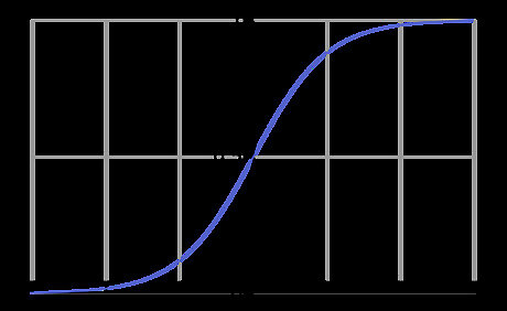
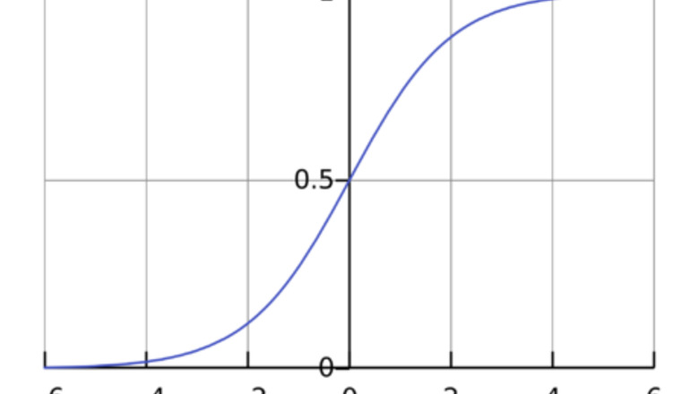
Solve for P {\displaystyle P} P. We let A = e C {\displaystyle A=e^{C}} A=e^{{C}} and recognize that it too is unaffected by the plus-minus sign, so we can discard it. ln ⁡ | L − P P | = − k t + C | L − P P | = e − k t + C L − P P = ± A e − k t L P − 1 = A e − k t P L = 1 A e − k t + 1 {\displaystyle {\begin{aligned}\ln \left|{\frac {L-P}{P}}\right|&=-kt+C\\\left|{\frac {L-P}{P}}\right|&=e^{-kt+C}\\{\frac {L-P}{P}}&=\pm Ae^{-kt}\\{\frac {L}{P}}-1&=Ae^{-kt}\\{\frac {P}{L}}&={\frac {1}{Ae^{-kt}+1}}\end{aligned}}} {\begin{aligned}\ln \left|{\frac {L-P}{P}}\right|&=-kt+C\\\left|{\frac {L-P}{P}}\right|&=e^{{-kt+C}}\\{\frac {L-P}{P}}&=\pm Ae^{{-kt}}\\{\frac {L}{P}}-1&=Ae^{{-kt}}\\{\frac {P}{L}}&={\frac {1}{Ae^{{-kt}}+1}}\end{aligned}} P = L A e − k t + 1 {\displaystyle P={\frac {L}{Ae^{-kt}+1}}} P={\frac {L}{Ae^{{-kt}}+1}} The above equation is the solution to the logistic growth problem, with a graph of the logistic curve shown. As expected of a first-order differential equation, we have one more constant A , {\displaystyle A,} A, which is determined by the initial population.

Bernoulli Equation

Write the logistic differential equation. Expand the right side and move the first order term to the left side. We can clearly see that this equation is nonlinear from the P 2 {\displaystyle P^{2}} P^{{2}} term. In general, nonlinear differential equations do not have solutions which can be written in terms of elementary functions, but the Bernoulli equation is an important exception. d P d t − k P = − k L P 2 {\displaystyle {\frac {\mathrm {d} P}{\mathrm {d} t}}-kP=-{\frac {k}{L}}P^{2}} {\frac {{\mathrm {d}}P}{{\mathrm {d}}t}}-kP=-{\frac {k}{L}}P^{{2}}

Multiply both sides by − P − 2 {\displaystyle -P^{-2}} -P^{{-2}}. When solving Bernoulli equations in general, we would multiply by ( 1 − n ) P − n , {\displaystyle (1-n)P^{-n},} (1-n)P^{{-n}}, where n {\displaystyle n} n denotes the degree of the nonlinear term. In our case, it is 2. − P − 2 d P d t + k P − 1 = k L {\displaystyle -P^{-2}{\frac {\mathrm {d} P}{\mathrm {d} t}}+kP^{-1}={\frac {k}{L}}} -P^{{-2}}{\frac {{\mathrm {d}}P}{{\mathrm {d}}t}}+kP^{{-1}}={\frac {k}{L}}

Rewrite the derivative term. We can apply the chain rule backwards to see that − P − 2 d P d t = d P − 1 d t . {\displaystyle -P^{-2}{\frac {\mathrm {d} P}{\mathrm {d} t}}={\frac {\mathrm {d} P^{-1}}{\mathrm {d} t}}.} -P^{{-2}}{\frac {{\mathrm {d}}P}{{\mathrm {d}}t}}={\frac {{\mathrm {d}}P^{{-1}}}{{\mathrm {d}}t}}. The equation is now linear in P − 1 . {\displaystyle P^{-1}.} P^{{-1}}. d P − 1 d t + k P − 1 = k L {\displaystyle {\frac {\mathrm {d} P^{-1}}{\mathrm {d} t}}+kP^{-1}={\frac {k}{L}}} {\frac {{\mathrm {d}}P^{{-1}}}{{\mathrm {d}}t}}+kP^{{-1}}={\frac {k}{L}}

Solve the equation for P − 1 {\displaystyle P^{-1}} P^{{-1}}. As standard for linear first order differential equations, we use the integrating factor e ∫ g ( x ) d x , {\displaystyle e^{\int g(x)\mathrm {d} x},} e^{{\int g(x){\mathrm {d}}x}}, where g ( x ) {\displaystyle g(x)} g(x) is the coefficient of P − 1 , {\displaystyle P^{-1},} P^{{-1}}, to convert into an exact equation. Therefore, our integrating factor is e k t . {\displaystyle e^{kt}.} e^{{kt}}. e k t d P − 1 + ( k P − 1 − k L ) e k t d t = 0 {\displaystyle e^{kt}\mathrm {d} P^{-1}+\left(kP^{-1}-{\frac {k}{L}}\right)e^{kt}\mathrm {d} t=0} e^{{kt}}{\mathrm {d}}P^{{-1}}+\left(kP^{{-1}}-{\frac {k}{L}}\right)e^{{kt}}{\mathrm {d}}t=0 ∫ e k t d P − 1 = P − 1 e k t + R ( t ) {\displaystyle \int e^{kt}\mathrm {d} P^{-1}=P^{-1}e^{kt}+R(t)} \int e^{{kt}}{\mathrm {d}}P^{{-1}}=P^{{-1}}e^{{kt}}+R(t) R ( t ) = ∫ − k L e k t d t = − 1 L e k t {\displaystyle {\begin{aligned}R(t)&=\int -{\frac {k}{L}}e^{kt}\mathrm {d} t\\&=-{\frac {1}{L}}e^{kt}\end{aligned}}} {\begin{aligned}R(t)&=\int -{\frac {k}{L}}e^{{kt}}{\mathrm {d}}t\\&=-{\frac {1}{L}}e^{{kt}}\end{aligned}} 1 P e k t − 1 L e k t = C {\displaystyle {\frac {1}{P}}e^{kt}-{\frac {1}{L}}e^{kt}=C} {\frac {1}{P}}e^{{kt}}-{\frac {1}{L}}e^{{kt}}=C

Isolate P {\displaystyle P} P. We solved the differential equation, but it was linear in P − 1 , {\displaystyle P^{-1},} P^{{-1}}, so we have to take the reciprocal of our answer. 1 P − 1 L = C e − k t L − P P L = C e − k t L − P = P L C e − k t L = P ( 1 + L C e − k t ) {\displaystyle {\begin{aligned}{\frac {1}{P}}-{\frac {1}{L}}&=Ce^{-kt}\\{\frac {L-P}{PL}}&=Ce^{-kt}\\L-P&=PLCe^{-kt}\\L&=P(1+LCe^{-kt})\end{aligned}}} {\begin{aligned}{\frac {1}{P}}-{\frac {1}{L}}&=Ce^{{-kt}}\\{\frac {L-P}{PL}}&=Ce^{{-kt}}\\L-P&=PLCe^{{-kt}}\\L&=P(1+LCe^{{-kt}})\end{aligned}}

Arrive at the solution. Rewrite L C {\displaystyle LC} LC as a new constant A . {\displaystyle A.} A. P = L 1 + A e − k t {\displaystyle P={\frac {L}{1+Ae^{-kt}}}} P={\frac {L}{1+Ae^{{-kt}}}}