views
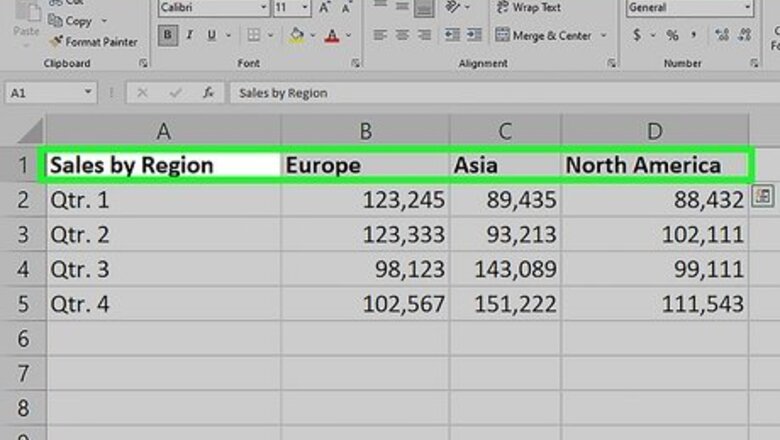
Select the data you want to transpose.
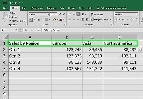
Click the first cell and drag to select the whole range. You can also select a single cell, hold down the ⇧ Shift key, and then use the arrow keys to select the range using your keyboard. Another option is to click one of the cells in the desired range, then hit ⌘ Command+A (on a Mac) or Ctrl+A (in Windows) to select the entire range.
Click Copy on the Home tab.
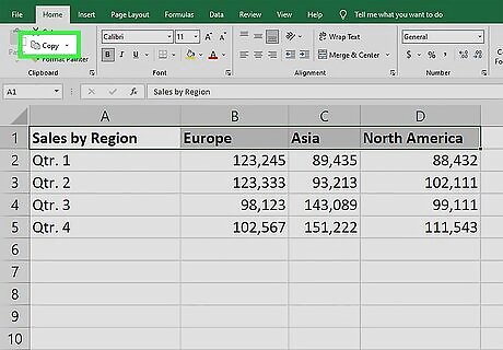
Find the Home tab at the top left corner of the window. Then, click the Copy button. You can also use the keyboard shortcut ⌘ Command+C on a Mac or Ctrl+C in Windows. Make sure you use the Copy command rather than the Cut command. Otherwise, you won’t be able to paste your data.
Select a cell where you’d like to paste the data.
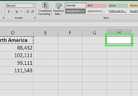
Choose a location that doesn’t overlap other data on the spreadsheet. Otherwise, the data you’re pasting will overwrite any data that’s currently occupying those cells. For instance, if you’re moving data from the row A:1-C:1, try clicking on E:2 to start your new column.
Open the Paste menu.
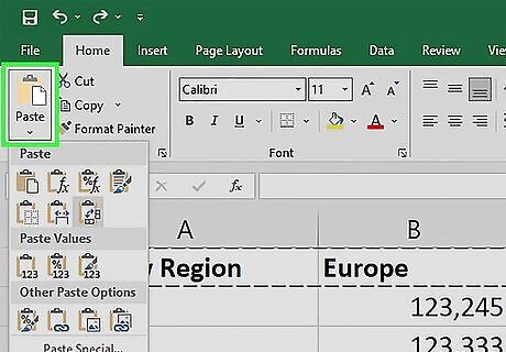
Navigate to the Home tab in the ribbon menu. Then, locate the Paste icon in the top left corner of the menu. It looks like a clipboard with a blank rectangle overlapping it. Click the down arrow next to the Paste icon to open a dropdown menu of paste options. Alternatively, right-click the top left portion of the cell where you want to paste your data to open a context menu. Or, if you’re on a Mac, ^ Control-click on the cell instead.
Click Transpose.
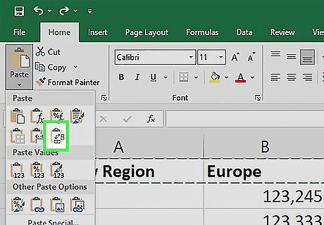
Locate Transpose in the list of paste options and click on it. This will paste your data to the new location you selected and automatically rotate it. That is, if your original data range was in rows, it will now appear as columns, and vice versa. Depending on which version of Excel you’re using, you may see the Transpose option as an icon that looks like a clipboard with 2 perpendicular blue and white rectangles connected by a curved arrow.
Delete the data in the original range if you like (optional).
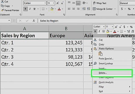
The original data will still appear in its old location. If you don’t need the data in both places, select the original range and delete it.
Make sure any formulas you transpose use absolute references.
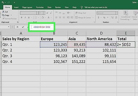
Locking your data references will ensure your formulas still work. If you have any formulas in your range that are linked to data located in other cells (relative references), the results may be skewed when you transpose the data. This is because the reference cell will shift when you move the data, so the formula will be drawing its data from a different location in the spreadsheet. To prevent this from happening: Add a dollar sign before the column and row references in each formula. For instance, if a cell contains the formula =A2+B3, change it to =$A$2+$B$3 to lock the reference and change the formula from relative to absolute. Add a dollar sign to just the row or just the column reference to create a “mixed” reference that is partially relative and partially absolute. For instance, =$A3 will lock the reference to column A, but not to row 3.
Convert tables to ranges before using the paste transpose feature.
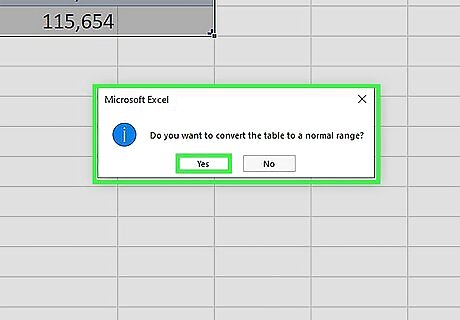
Tables won’t rotate properly using paste transpose. If you want to keep the data in your tables, you’ll have to convert them into ranges first. Select the table, then navigate to the Table tab in the ribbon menu. Click Convert to Range, then click Yes in the pop-up to confirm.
Use the TRANSPOSE function as an alternative to paste transpose.
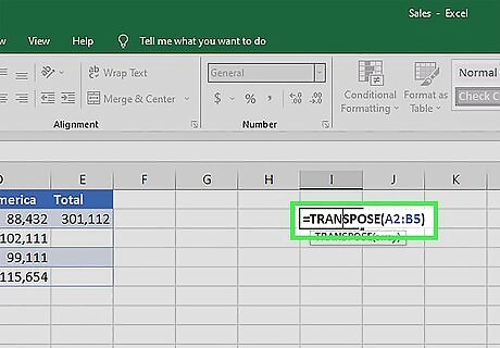
This command will also rotate the data in your tables. To use the TRANSPOSE function: Select a range of blank cells where you’d like your data to go, making sure it’s the same number of cells as the original range. In the first cell of your new range, type =TRANSPOSE(). Insert the original data range (e.g., A1:B6) in the parentheses. Hit Ctrl+⇧ Shift+↵ Enter. Your data, including any tables, will appear in the new range you selected.


Comments
0 comment