views
Tabulating Your Data
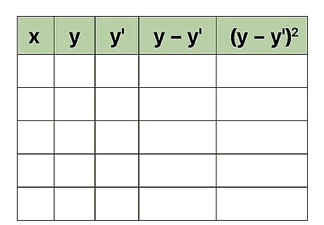
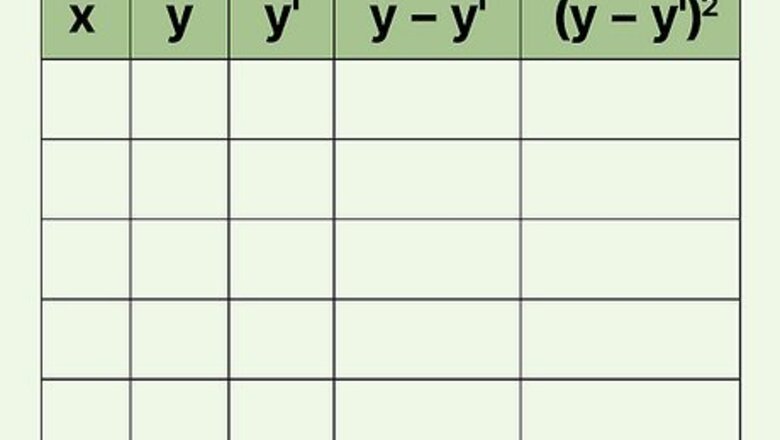
Create a five column data table. Any statistical work is generally made easier by having your data in a concise format. A simple table serves this purpose very well. To calculate the standard error of estimate, you will be using five different measurements or calculations. Therefore, creating a five-column table is helpful. Label the five columns as follows: x {\displaystyle x} x y {\displaystyle y} y y ′ {\displaystyle y^{\prime }} y^{{\prime }} y − y ′ {\displaystyle y-y^{\prime }} y-y^{{\prime }} ( y − y ′ ) 2 {\displaystyle (y-y^{\prime })^{2}} (y-y^{{\prime }})^{2} Note that the table shown in the image above performs the opposite subtractions, y ′ − y {\displaystyle y^{\prime }-y} y^{{\prime }}-y. The more standard order, however, is y − y ′ {\displaystyle y-y^{\prime }} y-y^{{\prime }}. Because the values in the final column are squared, the negative is not problematic and will not change the outcome. Nevertheless, you should recognize that the more standard calculation is y − y ′ {\displaystyle y-y^{\prime }} y-y^{{\prime }}.
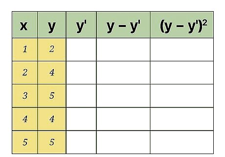
Enter the data values for your measured data. After collecting your data, you will have pairs of data values. For these statistical calculations, the independent variable is labeled x {\displaystyle x} x and the dependent, or resulting, variable is y {\displaystyle y} y. Enter these values into the first two columns of your data table. The order of the data and the pairing is important for these calculations. You need to be careful to keep your paired data points together in order. For the sample calculations shown above, the data pairs are as follows: (1,2) (2,4) (3,5) (4,4) (5,5)
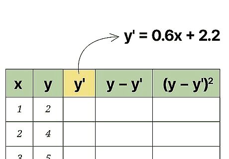
Calculate a regression line. Using your data results, you will be able to calculate a regression line. This is also called a line of best fit or the least squares line. The calculation is tedious but can be done by hand. Alternatively, you can use a handheld graphing calculator or some online programs that will quickly calculate a best fit line using your data. For this article, it is assumed that you will have the regression line equation available or that it has been predicted by some prior means. For the sample data set in the image above, the regression line is y ′ = 0.6 x + 2.2 {\displaystyle y^{\prime }=0.6x+2.2} y^{{\prime }}=0.6x+2.2.
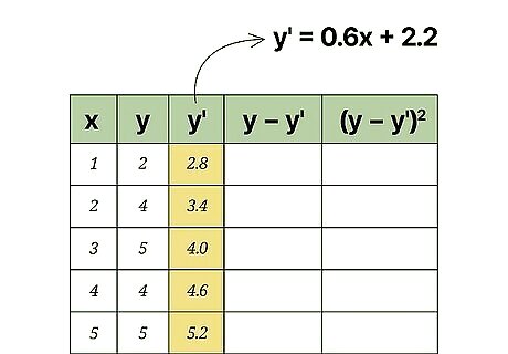
Calculate predicted values from the regression line. Using the equation of that line, you can calculate predicted y-values for each x-value in your study, or for other theoretical x-values that you did not measure. Using the equation of the regression line, calculate or “predict” values of y ′ {\displaystyle y^{\prime }} y^{{\prime }} for each value of x. Insert the x-value into the equation, and find the result for y ′ {\displaystyle y^{\prime }} y^{{\prime }} as follows: y ′ = 0.6 x + 2.2 {\displaystyle y^{\prime }=0.6x+2.2} y^{{\prime }}=0.6x+2.2 y ′ ( 1 ) = 0.6 ( 1 ) + 2.2 = 2.8 {\displaystyle y^{\prime }(1)=0.6(1)+2.2=2.8} y^{{\prime }}(1)=0.6(1)+2.2=2.8 y ′ ( 2 ) = 0.6 ( 2 ) + 2.2 = 3.4 {\displaystyle y^{\prime }(2)=0.6(2)+2.2=3.4} y^{{\prime }}(2)=0.6(2)+2.2=3.4 y ′ ( 3 ) = 0.6 ( 3 ) + 2.2 = 4.0 {\displaystyle y^{\prime }(3)=0.6(3)+2.2=4.0} y^{{\prime }}(3)=0.6(3)+2.2=4.0 y ′ ( 4 ) = 0.6 ( 4 ) + 2.2 = 4.6 {\displaystyle y^{\prime }(4)=0.6(4)+2.2=4.6} y^{{\prime }}(4)=0.6(4)+2.2=4.6 y ′ ( 5 ) = 0.6 ( 5 ) + 2.2 = 5.2 {\displaystyle y^{\prime }(5)=0.6(5)+2.2=5.2} y^{{\prime }}(5)=0.6(5)+2.2=5.2
Performing the Calculations
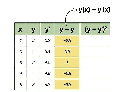
Calculate the error of each predicted value. In the fourth column of your data table, you will calculate and record the error of each predicted value. Specifically, subtract the predicted value ( y ′ {\displaystyle y^{\prime }} y^{{\prime }}) from the actual observed value ( y {\displaystyle y} y). For the data in the sample set, these calculations are as follows: y ( x ) − y ′ ( x ) {\displaystyle y(x)-y^{\prime }(x)} y(x)-y^{{\prime }}(x) y ( 1 ) − y ′ ( 1 ) = 2 − 2.8 = − 0.8 {\displaystyle y(1)-y^{\prime }(1)=2-2.8=-0.8} y(1)-y^{{\prime }}(1)=2-2.8=-0.8 y ( 2 ) − y ′ ( 2 ) = 4 − 3.4 = 0.6 {\displaystyle y(2)-y^{\prime }(2)=4-3.4=0.6} y(2)-y^{{\prime }}(2)=4-3.4=0.6 y ( 3 ) − y ′ ( 3 ) = 5 − 4 = 1 {\displaystyle y(3)-y^{\prime }(3)=5-4=1} y(3)-y^{{\prime }}(3)=5-4=1 y ( 4 ) − y ′ ( 4 ) = 4 − 4.6 = − 0.6 {\displaystyle y(4)-y^{\prime }(4)=4-4.6=-0.6} y(4)-y^{{\prime }}(4)=4-4.6=-0.6 y ( 5 ) − y ′ ( 5 ) = 5 − 5.2 = − 0.2 {\displaystyle y(5)-y^{\prime }(5)=5-5.2=-0.2} y(5)-y^{{\prime }}(5)=5-5.2=-0.2
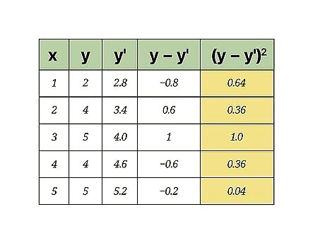
Calculate the squares of the errors. Take each value in the fourth column and square it by multiplying it by itself. Fill in these results in the final column of your data table. For the sample data set, these calculations are as follows: − 0.8 2 = 0.64 {\displaystyle -0.8^{2}=0.64} -0.8^{2}=0.64 0.6 2 = 0.36 {\displaystyle 0.6^{2}=0.36} 0.6^{2}=0.36 1 2 = 1.0 {\displaystyle 1^{2}=1.0} 1^{2}=1.0 − 0.6 = 0.36 {\displaystyle -0.6=0.36} -0.6=0.36 − 0.2 = 0.04 {\displaystyle -0.2=0.04} -0.2=0.04
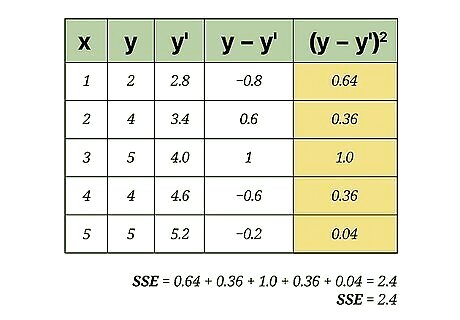
Find the sum of the squared errors (SSE). The statistical value known as the sum of squared errors (SSE) is a useful step in finding standard deviation, variance and other measurements. To find the SSE from your data table, add the values in the fifth column of your data table. For this sample data set, this calculation is as follows: 0.64 + 0.36 + 1.0 + 0.36 + 0.04 = 2.4 {\displaystyle 0.64+0.36+1.0+0.36+0.04=2.4} 0.64+0.36+1.0+0.36+0.04=2.4
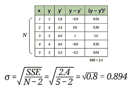
Finalize your calculations. The Standard Error of the Estimate is the square root of the average of the SSE. It is generally represented with the Greek letter σ {\displaystyle \sigma } \sigma . Therefore, the first calculation is to divide the SSE score by the number of measured data points. Then, find the square root of that result. If the measured data represents an entire population, then you will find the average by dividing by N, the number of data points. However, if you are working with a smaller sample set of the population, then substitute N-2 in the denominator. For the sample data set in this article, we can assume that it is a sample set and not a population, just because there are only 5 data values. Therefore, calculate the Standard Error of the Estimate as follows: σ = 2.4 5 − 2 {\displaystyle \sigma ={\sqrt {\frac {2.4}{5-2}}}} \sigma ={\sqrt {{\frac {2.4}{5-2}}}} σ = 2.4 3 {\displaystyle \sigma ={\sqrt {\frac {2.4}{3}}}} \sigma ={\sqrt {{\frac {2.4}{3}}}} σ = 0.8 {\displaystyle \sigma ={\sqrt {0.8}}} \sigma ={\sqrt {0.8}} σ = 0.894 {\displaystyle \sigma =0.894} \sigma =0.894
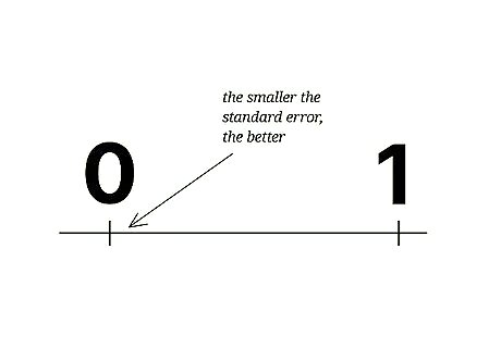
Interpret your result. The Standard Error of the Estimate is a statistical figure that tells you how well your measured data relates to a theoretical straight line, the line of regression. A score of 0 would mean a perfect match, that every measured data point fell directly on the line. Widely scattered data will have a much higher score. With this small sample set, the standard error score of 0.894 is quite low and represents well organized data results.


Comments
0 comment