
Finding the Correlation Coefficient by Hand
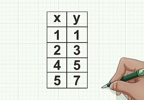
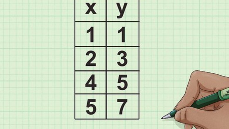
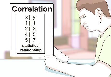
Assemble your data. To begin calculating a correlation efficient, first examine your data pairs. It is helpful to put them in a table, either vertically or horizontally. Label each row or column x and y. For example, suppose you have four data pairs for x and y. Your table may look like this: x || y 1 || 1 2 || 3 4 || 5 5 || 7
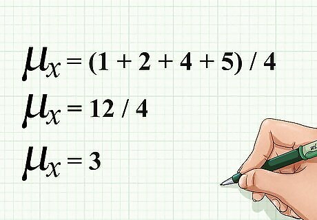
Calculate the mean of x. In order to calculate the mean, you must add all the values of x, then divide by the number of values. Using the example above, note that you have four values for x. To calculate the mean, add all the values given for x, then divide by 4. Your calculation would look like this: μ x = ( 1 + 2 + 4 + 5 ) / 4 {\displaystyle \mu _{x}=(1+2+4+5)/4} \mu _{x}=(1+2+4+5)/4 μ x = 12 / 4 {\displaystyle \mu _{x}=12/4} \mu _{x}=12/4 μ x = 3 {\displaystyle \mu _{x}=3} \mu _{x}=3

Find the mean of y. To find the mean of y, follow the same steps, adding all the values of y together, then dividing by the number of values. In the example above, you also have four values for y. Add all these values, then divide by 4. Your calculations would look like this: μ y = ( 1 + 3 + 5 + 7 ) / 4 {\displaystyle \mu _{y}=(1+3+5+7)/4} \mu _{y}=(1+3+5+7)/4 μ y = 16 / 4 {\displaystyle \mu _{y}=16/4} \mu _{y}=16/4 μ y = 4 {\displaystyle \mu _{y}=4} \mu _{y}=4
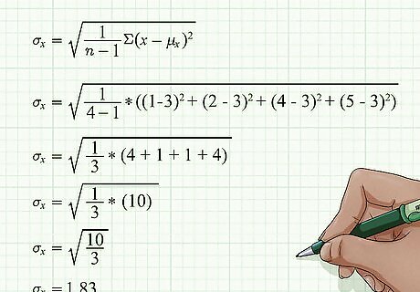
Determine the standard deviation of x. Once you have your means, you can calculate standard deviation. To do so, use the formula: σ x = 1 n − 1 Σ ( x − μ x ) 2 {\displaystyle \sigma _{x}={\sqrt {{\frac {1}{n-1}}\Sigma (x-\mu _{x})^{2}}}} \sigma _{x}={\sqrt {{\frac {1}{n-1}}\Sigma (x-\mu _{x})^{2}}} With the sample data, your calculations should look like this: σ x = 1 4 − 1 ∗ ( ( 1 − 3 ) 2 + ( 2 − 3 ) 2 + ( 4 − 3 ) 2 + ( 5 − 3 ) 2 ) {\displaystyle \sigma _{x}={\sqrt {{\frac {1}{4-1}}*((1-3)^{2}+(2-3)^{2}+(4-3)^{2}+(5-3)^{2})}}} \sigma _{x}={\sqrt {{\frac {1}{4-1}}*((1-3)^{2}+(2-3)^{2}+(4-3)^{2}+(5-3)^{2})}} σ x = 1 3 ∗ ( 4 + 1 + 1 + 4 ) {\displaystyle \sigma _{x}={\sqrt {{\frac {1}{3}}*(4+1+1+4)}}} \sigma _{x}={\sqrt {{\frac {1}{3}}*(4+1+1+4)}} σ x = 1 3 ∗ ( 10 ) {\displaystyle \sigma _{x}={\sqrt {{\frac {1}{3}}*(10)}}} \sigma _{x}={\sqrt {{\frac {1}{3}}*(10)}} σ x = 10 3 {\displaystyle \sigma _{x}={\sqrt {\frac {10}{3}}}} \sigma _{x}={\sqrt {{\frac {10}{3}}}} σ x = 1.83 {\displaystyle \sigma _{x}=1.83} \sigma _{x}=1.83
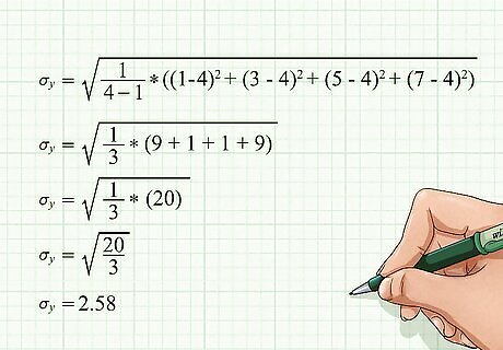
Calculate the standard deviation of y. Using the same basic steps, find the standard deviation of y. You will use the same formula, using the y data points. With the sample data, your calculations should look like this: σ y = 1 4 − 1 ∗ ( ( 1 − 4 ) 2 + ( 3 − 4 ) 2 + ( 5 − 4 ) 2 + ( 7 − 4 ) 2 ) {\displaystyle \sigma _{y}={\sqrt {{\frac {1}{4-1}}*((1-4)^{2}+(3-4)^{2}+(5-4)^{2}+(7-4)^{2})}}} \sigma _{y}={\sqrt {{\frac {1}{4-1}}*((1-4)^{2}+(3-4)^{2}+(5-4)^{2}+(7-4)^{2})}} σ y = 1 3 ∗ ( 9 + 1 + 1 + 9 ) {\displaystyle \sigma _{y}={\sqrt {{\frac {1}{3}}*(9+1+1+9)}}} \sigma _{y}={\sqrt {{\frac {1}{3}}*(9+1+1+9)}} σ y = 1 3 ∗ ( 20 ) {\displaystyle \sigma _{y}={\sqrt {{\frac {1}{3}}*(20)}}} \sigma _{y}={\sqrt {{\frac {1}{3}}*(20)}} σ y = 20 3 {\displaystyle \sigma _{y}={\sqrt {\frac {20}{3}}}} \sigma _{y}={\sqrt {{\frac {20}{3}}}} σ y = 2.58 {\displaystyle \sigma _{y}=2.58} \sigma _{y}=2.58
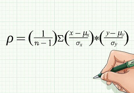
Review the basic formula for finding a correlation coefficient. The formula for calculating a correlation coefficient uses means, standard deviations, and the number of pairs in your data set (represented by n). The correlation coefficient itself is represented by the lower-case letter r or the lower-case Greek letter rho, ρ. For this article, you will use the formula known as the Pearson correlation coefficient, shown below: ρ = ( 1 n − 1 ) Σ ( x − μ x σ x ) ∗ ( y − μ y σ y ) {\displaystyle \rho =\left({\frac {1}{n-1}}\right)\Sigma \left({\frac {x-\mu _{x}}{\sigma _{x}}}\right)*\left({\frac {y-\mu _{y}}{\sigma _{y}}}\right)} \rho =\left({\frac {1}{n-1}}\right)\Sigma \left({\frac {x-\mu _{x}}{\sigma _{x}}}\right)*\left({\frac {y-\mu _{y}}{\sigma _{y}}}\right) You may notice slight variations in the formula, here or in other texts. For example, some will use the Greek notation with rho and sigma, while others will use r and s. Some texts may show slightly different formulas; but they will be mathematically equivalent to this one.
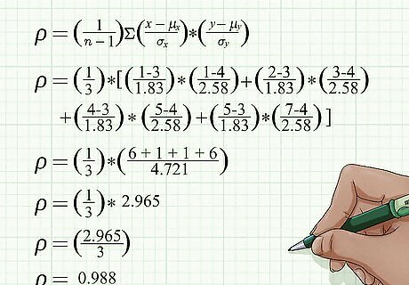
Find the correlation coefficient. You now have the means and standard deviations for your variables, so you can proceed to use the correlation coefficient formula. Remember that n represents the number of values you have. You have already worked out the other relevant information in the steps above. Using the sample data, you would enter your data in the correlation coefficient formula and calculate as follows: ρ = ( 1 n − 1 ) Σ ( x − μ x σ x ) ∗ ( y − μ y σ y ) {\displaystyle \rho =\left({\frac {1}{n-1}}\right)\Sigma \left({\frac {x-\mu _{x}}{\sigma _{x}}}\right)*\left({\frac {y-\mu _{y}}{\sigma _{y}}}\right)} \rho =\left({\frac {1}{n-1}}\right)\Sigma \left({\frac {x-\mu _{x}}{\sigma _{x}}}\right)*\left({\frac {y-\mu _{y}}{\sigma _{y}}}\right) ρ = ( 1 3 ) ∗ {\displaystyle \rho =\left({\frac {1}{3}}\right)*} \rho =\left({\frac {1}{3}}\right)*[ ( 1 − 3 1.83 ) ∗ ( 1 − 4 2.58 ) + ( 2 − 3 1.83 ) ∗ ( 3 − 4 2.58 ) {\displaystyle \left({\frac {1-3}{1.83}}\right)*\left({\frac {1-4}{2.58}}\right)+\left({\frac {2-3}{1.83}}\right)*\left({\frac {3-4}{2.58}}\right)} \left({\frac {1-3}{1.83}}\right)*\left({\frac {1-4}{2.58}}\right)+\left({\frac {2-3}{1.83}}\right)*\left({\frac {3-4}{2.58}}\right) + ( 4 − 3 1.83 ) ∗ ( 5 − 4 2.58 ) + ( 5 − 3 1.83 ) ∗ ( 7 − 4 2.58 ) {\displaystyle +\left({\frac {4-3}{1.83}}\right)*\left({\frac {5-4}{2.58}}\right)+\left({\frac {5-3}{1.83}}\right)*\left({\frac {7-4}{2.58}}\right)} +\left({\frac {4-3}{1.83}}\right)*\left({\frac {5-4}{2.58}}\right)+\left({\frac {5-3}{1.83}}\right)*\left({\frac {7-4}{2.58}}\right)] ρ = ( 1 3 ) ∗ ( 6 + 1 + 1 + 6 4.721 ) {\displaystyle \rho =\left({\frac {1}{3}}\right)*\left({\frac {6+1+1+6}{4.721}}\right)} \rho =\left({\frac {1}{3}}\right)*\left({\frac {6+1+1+6}{4.721}}\right) ρ = ( 1 3 ) ∗ 2.965 {\displaystyle \rho =\left({\frac {1}{3}}\right)*2.965} \rho =\left({\frac {1}{3}}\right)*2.965 ρ = ( 2.965 3 ) {\displaystyle \rho =\left({\frac {2.965}{3}}\right)} \rho =\left({\frac {2.965}{3}}\right) ρ = 0.988 {\displaystyle \rho =0.988} \rho =0.988
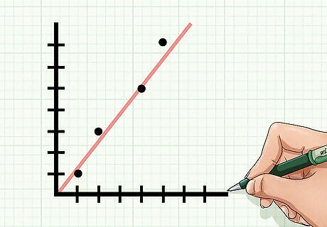
Interpret your result. For this data set, the correlation coefficient is 0.988. This number tells you two things about the data. Look at the sign of the number and the size of the number. Because the correlation coefficient is positive, you can say there is a positive correlation between the x-data and the y-data. This means that as the x values increase, you expect the y values to increase also. Because the correlation coefficient is very close to +1, the x-data and y-data are very closely connected. If you were to graph these points, you would see that they form a very good approximation of a straight line.
Using Online Correlation Calculators

Search the Internet for correlation calculators. Measuring correlation is a fairly standard calculation for statisticians. The calculation can become very tedious if done by hand for large data sets. As a result, many sources have made correlation calculators available online. Use any search engine and enter the search term “correlation calculator.”
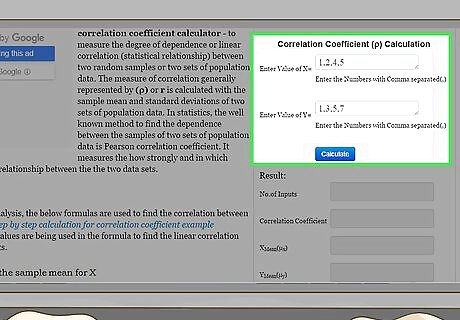
Enter your data. Carefully review the instructions on the website so you will enter your data properly. It is important that your data pairs are kept in order, or you will generate an incorrect correlation result. Different websites use different formats to enter data. For example, at the website http://ncalculators.com/statistics/correlation-coefficient-calculator.htm, you will find one horizontal box for entering x-values and a second horizontal box for entering y-values. You enter your terms, separated only by commas. Thus, the x-data set that was calculated earlier in this article should be entered as 1,2,4,5. The y-data set should be 1,3,5,7. At another site, http://www.alcula.com/calculators/statistics/correlation-coefficient/, you can enter data either horizontally or vertically, as long as you keep the data points in order.
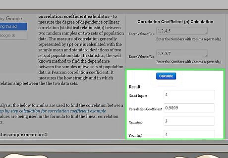
Calculate your results. These calculation sites are popular because, after you enter your data, you generally need only to click on the button that says “Calculate,” and the result will appear automatically.
Using Graphing Calculators
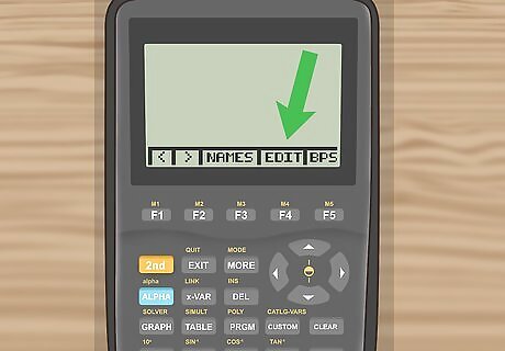
Enter your data. Using a handheld graphing calculator, enter your calculator’s statistics function and then select the “Edit” command. Each calculator will have slightly different key commands. This article will give the specific instructions for the Texas Instruments TI-86. Enter the Stat function by pressing [2nd]-Stat (above the + key), then hit F2-Edit.
Clear any old stored data. Most calculators will keep statistical data until cleared. To make sure that you do not confuse old data with new data, you should first clear any previously stored information. Use the arrow keys to move the cursor to highlight the heading “xStat.” Then press Clear and Enter. This should clear all values in the xStat column. Use the arrow keys to highlight the yStat heading. Press Clear and Enter to empty the data from that column as well.
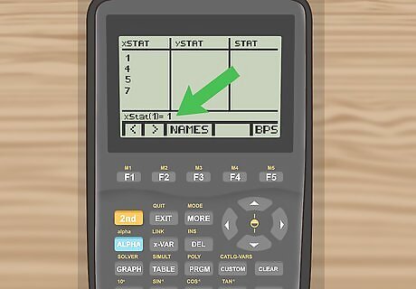
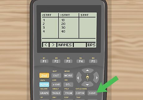
Enter your data values. Using the arrow keys, move the cursor to the first space under the xStat heading. Type in your first data value and then hit Enter. You should see the space at the bottom of the screen display “xStat(1)=__,” with your value filling the blank space. When you hit Enter, the data will fill the table, the cursor will move to the next line, and the line at the bottom of the screen should now read “xStat(2)=__.” Continue entering all the x-data values. When you complete the x-data, use the arrow keys to move to the yStat column and enter the y-data values. After all the data has been entered, hit Exit to clear the screen and leave the Stat menu.
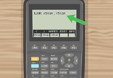
Calculate the linear regression statistics. The correlation coefficient is a measure of how well the data approximates a straight line. A statistical graphing calculator can very quickly calculate the best-fit line and the correlation coefficient. Enter the Stat function and then hit the Calc button. On the TI-86, this is [2nd][Stat][F1]. Choose the Linear Regression calculations. On the TI-86, this is [F3], which is labeled “LinR.” The graphic screen should then display the line “LinR _,” with a blinking cursor. You now need to enter the names of the two variables that you want to calculate. These are xStat and yStat. On the TI-86, select the Names list by hitting [2nd][List][F3]. The bottom line of your screen should now show the available variables. Choose [xStat] (this is probably button F1 or F2), then enter a comma, then [yStat]. Hit Enter to calculate the data.
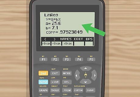
Interpret your results. When you hit Enter, the calculator will instantly calculate the following information for the data that you entered: y = a + b x {\displaystyle y=a+bx} y=a+bx : This is the general formula for a straight line. However, instead of the familiar “y=mx+b,” this is presented in reverse order. a = {\displaystyle a=} a=. This is the value of the y-intercept of the best-fit line. b = {\displaystyle b=} b=. This is the slope of the best-fit line. corr = {\displaystyle {\text{corr}}=} {\text{corr}}=. This is the correlation coefficient. n = {\displaystyle n=} n=. This is the number of data pairs that were used in the calculation.
Reviewing the Fundamentals
Understand the concept of correlation. Correlation refers to the statistical relationship between two quantities. The correlation coefficient is a single number that you can calculate for any two sets of data points. The number will always be something between -1 and +1, and it indicates how closely connected the two data sets tend to be. For example, if you were to measure the heights and ages of children up to the age of about 12, you would expect to find a strong positive correlation. As children get older, they tend to get taller. An example of negative correlation would be data comparing a person’s time spent practicing golf shots and that person’s golf score. As the practice increases, the score should decrease. Finally, you would expect very little correlation, either positive or negative, between a person’s shoe size, for example, and SAT scores.
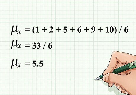
Know how to find a mean. The arithmetic mean, or “average,” of a set of data is calculated by adding all of the values of the data together, then dividing by the number of values in the set. When you find the correlation coefficient for your data, you will need to calculate the mean of each set of data. The mean of a variable is denoted by the variable with a horizontal line above it. This is often referred to as “x-bar” or “y-bar” for the x and y data sets. Alternatively, the mean may be signified by the lower-case Greek letter mu, μ. To indicate the mean of x-data points, for example, you could write μx or μ(x). As an example, if you have a set of x-data points (1,2,5,6,9,10), then the mean of this data is calculated as follows: μ x = ( 1 + 2 + 5 + 6 + 9 + 10 ) / 6 {\displaystyle \mu _{x}=(1+2+5+6+9+10)/6} \mu _{x}=(1+2+5+6+9+10)/6 μ x = 33 / 6 {\displaystyle \mu _{x}=33/6} \mu _{x}=33/6 μ x = 5.5 {\displaystyle \mu _{x}=5.5} \mu _{x}=5.5
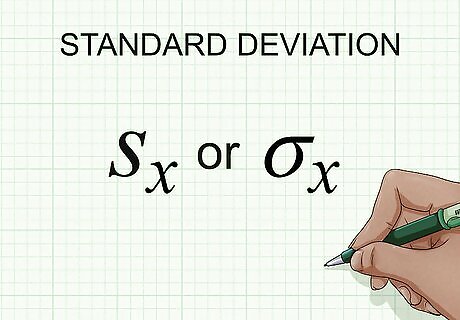
Note the importance of standard deviation. In statistics, standard deviation measures variation, showing how numbers are spread out in relationship to the mean. A group of numbers with a low standard deviation are fairly tightly collected. A group of numbers with a high standard deviation are widely scattered. Symbolically, standard deviation is expressed with either the lower-case letter s or the lower-case Greek letter sigma, σ. Thus, the standard deviation of the x-data is written as either sx or σx.
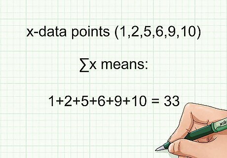
Recognize summation notation. The summation operator is one of the most common operators in mathematics, indicating a sum of values. It is represented by the upper-case Greek letter, sigma, or ∑. As an example, if you have a set of x-data points (1,2,5,6,9,10), then ∑x means: 1+2+5+6+9+10 = 33.


Comments
0 comment